Excel waterfall chart with multiple series
Excel Waterfall Charts Bridge Charts. Now click on Insert Tab from the top of the Excel window and then select Insert Line or Area Chart.
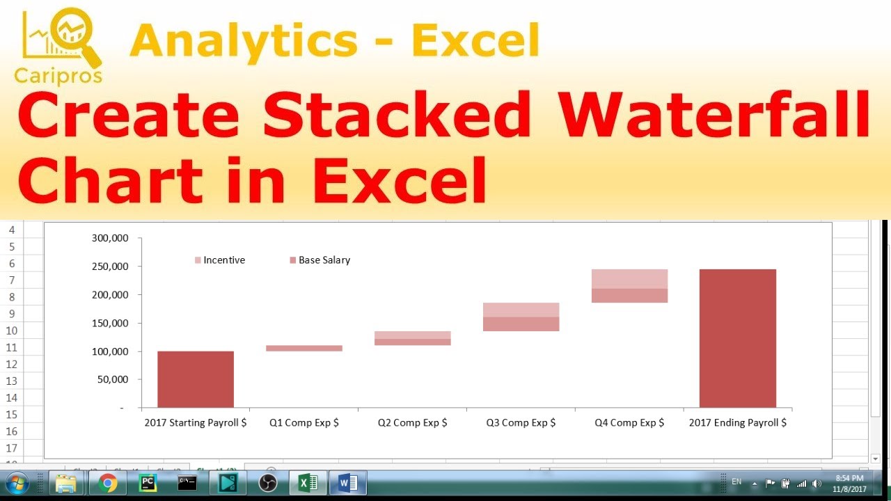
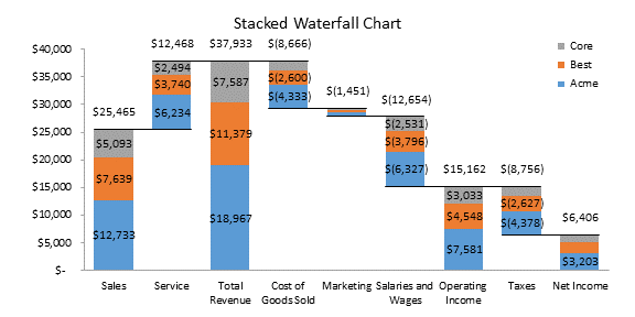
Excel Chart Stacked Waterfall Chart For Annual Expenses Reporting Youtube
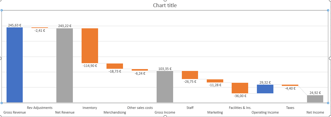
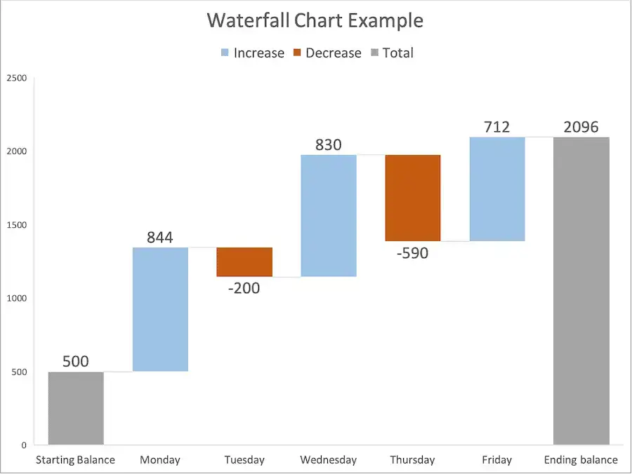
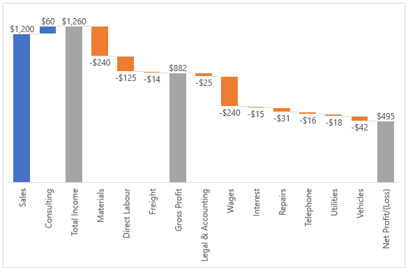
A waterfall chart also known as a cascade chart or a bridge chart is a special kind of chart that illustrates how positive or negative values in a data series contribute to the totalIn other words its an ideal way to visualize a starting value the positive and negative changes made to that value and the resulting end value.
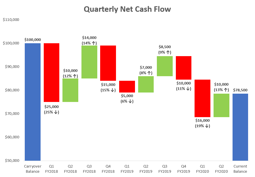
. Here we are considering two years sales as shown below for the products X Y and Z. Go to Insert Click the Recommended Charts icon. In simple terms it is the net impact of the organizations cash inflow and cash outflow for a particular period say monthly quarterly.
Following is an example of a doughnut chart in excel. Choose the Stock option. Now fill in the details for the Start The Base value will be similar to Net Cash Flow Net Cash Flow Net cash flow refers to the difference in cash inflows and outflows generated or lost over the period from all business activities combined.
From the pop-down menu select the first 2-D Line. This button appears on the right of your chart as soon as you click on it. I also make one of those add-ins.
If you prefer to read instead of. A Microsoft Excel template is especially convenient if you dont have a lot of experience making waterfall charts. To delete a certain data series from the chart permanently select that series and click the Remove bottom.
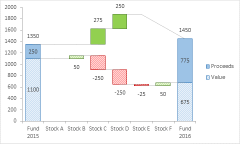
In our example Qtr_04 series default values are in E2E6. The easiest way to assemble a waterfall chart in Excel is to use a premade template. I have a tutorial for regular waterfall charts.
Check Values From Cells. This is a Comparison Chart in Excel. The table below shows the four series I need to make two series appear on the chart.
In my example I plot one series on the primary axis and one on the secondary series. From the pop-down menu select the first 2-D Line. Select chart data labels and right-click then choose Format Data Labels.
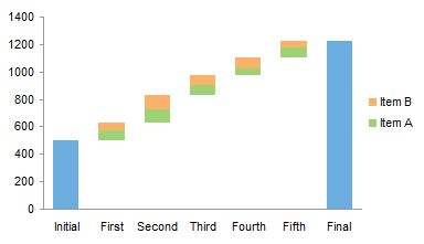
A clustered bar chart is a bar chart in excel Bar Chart In Excel Bar charts in excel are helpful in the representation of the single data on the horizontal bar with categories displayed on the Y-axis and values on the X-axis. The first and the last columns in a typical waterfall chart represent total values. All you need to do is to enter your data into the table and the Excel waterfall chart will automatically reflect the changes.
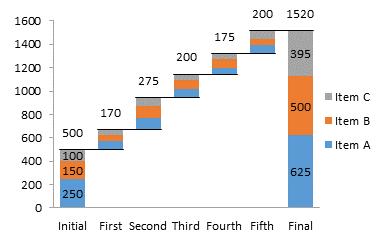
Hide or show series using the Charts Filter button. If you use the stacked column approach a stacked waterfall has multiple items per category. Double Doughnut Chart in Excel.
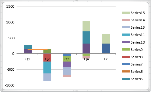
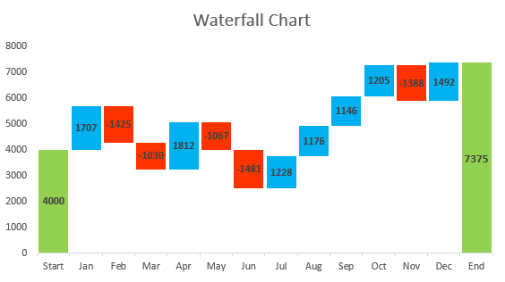
It uses simple but unusual techniques to quickly and easily get a Waterfall Chart that also works with negative cumulative values. If the order does not match your chart will not display properly and you will need to edit the Chart Data once the chart is created. You can also go through our other suggested articles.
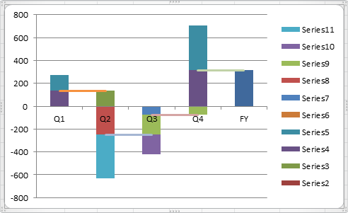
Watch the video to learn how to create a Waterfall or Bridge Chart in Excel. If you can make it work with one set of values you should be able to add one or more extra series to stack on the first. A waterfall chart is actually a special type of Excel column chart.
Pick Open-High-Low-Close See note below Click OK. Read more which represents data virtually in horizontal bars in series. Displaying multiple time series in an Excel chart is not difficult if all the series use the same dates but it becomes a problem if the dates are different for example if the series show monthly and.
Doughnut Chart in Excel Example 2. It is normally used to demonstrate how the starting position either increases or decreases through a series of changes. Waterfall charts 101.
I recently showed several ways to display Multiple Series in One Excel ChartThe current article describes a special case of this in which the X values are dates. Above step popup an input box for the user to select a range of cells to display on the chart instead of default values. Lets take an example of sales of a company.
With the help of a double doughnut chart we can show the two matrices in our chart. Comparison Charts are also known with a famous name as Multiple Column Chart or Multiple Bar Chart. Another way to manage the data series displayed in your Excel chart is using the Chart Filters button.
Select your chart data. Here we discuss how to create a comparison chart in Excel together with practical examples and an Excel template for download. For the dual axis chart I need the primary series data and blank data for the primary axis and I need blank data and the secondary series data for the secondary axis.
To create a bar chart we need at least two independent and dependent variables.
How To Create Waterfall Charts In Excel Page 5 Of 6 Excel Tactics

How To Create A Waterfall Chart In Excel
Excel Waterfall Charts Bridge Charts Peltier Tech
The New Waterfall Chart In Excel 2016 Peltier Tech

Stacked Waterfall Chart With Positive And Negative Values In Excel Super User
How To Create Waterfall Charts In Excel Page 5 Of 6 Excel Tactics
Excel Waterfall Chart How To Create One That Doesn T Suck
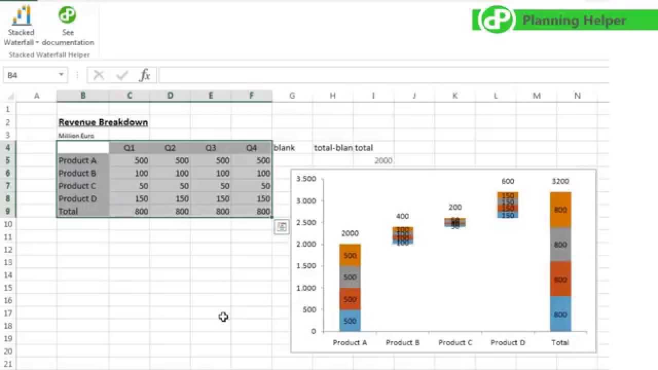
Stacked Waterfall Chart In 10 Seconds With A Free Add In For Excel Youtube
Excel Waterfall Charts Bridge Charts Peltier Tech
.png)
Waterfall Chart Excel Template How To Tips Teamgantt

Create Waterfall Or Bridge Chart In Excel
How To Set The Total Bar In An Excel Waterfall Chart Analyst Answers
The New Waterfall Chart In Excel 2016 Peltier Tech

Stacked Waterfall Chart Microsoft Power Bi Community
How To Create A Waterfall Chart In Excel Automate Excel
How To Create Waterfall Chart In Excel 2016 2013 2010
Excel Waterfall Charts My Online Training Hub